CausalCCC integration with NicheNet demo dataset
This vignette present the workflow performed to reconstruct a CausalCCC network using NicheNet cell-cell communication analysis on their demo dataset (see other tutorials). If you need more details about the CausalCCC helper functions presented here, we recommend you read the tutorials.
You can download their demo dataset here (Seurat object).
Setting up libraries
Make sure you can load the following packages :
### Mandatory Libraries
library(Seurat)
library(SeuratObject)
library(ggplot2)
library(tidyverse)
library(data.table)
library(dplyr)
library(igraph)

### For CCC selection - optional if you want to use your own L-R list
library(nichenetr) # Please update to v2.0.4
library(liana)

### For network aesthetic display
library(rjson)

#How to download CausalCCC
# CausalCCC is a module part of the miic R package
# Sys.setenv(GITHUB_PAT = 'YOUR_GITHUB_API_TOKEN_HERE')
# devtools::install_github("interactMIIC/causalCCC/miic_R_package", force = T) #latest version of MIIC
library(miic)


wd_path <- "~/CausalCCC/case_studies/NicheNet"
setwd(wd_path)
Initialization
The beginning of this analysis uses NicheNet scripts to perform cell-cell communication analysis.
Load your Seurat Object:
# Set your working directory here
seuratObj <- readRDS(file.path(wd_path,"data_nichenet/seuratObj.rds"))
seuratObj <- UpdateSeuratObject(seuratObj)
seuratObj <- alias_to_symbol_seurat(seuratObj, "mouse")
DimPlot(seuratObj, reduction = "tsne")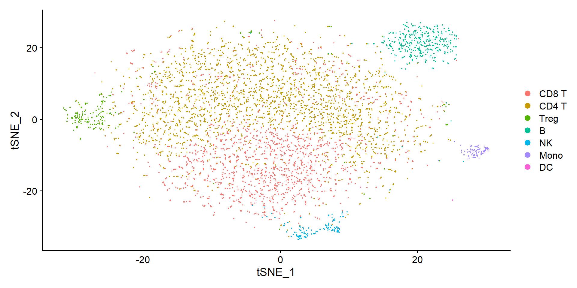
# Precise assay of interest
assay_name <- 'RNA'

# Specify the species genes format (mouse or human)
species <- "mouse"

# Define your senders, your receivers and the metadata where they can be found
senders <-  c("CD4 T")
receivers <-  c("CD8 T")
interact_ident <- "celltype"

# If you want to remove ribomosomal genes exectute this chunk:
ribomosal_genes <- row.names(seuratObj)[stringr::str_detect(row.names(seuratObj), ifelse(species == "human", "RPL|RPS","Rpl|Rps") )]
counts <- GetAssayData(seuratObj, assay = "RNA")
counts <- counts[-(which(rownames(counts) %in% ribomosal_genes)),]
seuratObj <- subset(seuratObj, features = rownames(counts))
rm(counts)
NicheNet Ligand-Receptor links
The first step is to get what we call CCC links (for Cell-Cell Communication links). This will get us the ligands and receptors genes to base the network reconstruction on. Which L-R interactions do you wish to get intracellular insights from ?
There are 3 main possible methods : - Find your own L-R links you want to investigate from expertise - Use the CCC method or statistical analysis of choice, here we showcase NicheNet - Use our integration of the LIANA pipeline, that can run a set of different methods
At the end, you should have a dataframe with a column ligands and a column receptors listing the L-R links. A third column “weight” can be added if your method outputs a quantitative measure of these L-R links. From this, you easily obtain a ligands vector and a receptors vector.
We use NicheNet to obtain the CCC links. Please note that this is mostly referencing the code from their vignette.
Click here to show the code
## Set up
organism <- "mouse"

if(organism == "human"){
  lr_network <- readRDS(url("https://zenodo.org/record/7074291/files/lr_network_human_21122021.rds"))
  ligand_target_matrix <- readRDS(url("https://zenodo.org/record/7074291/files/ligand_target_matrix_nsga2r_final.rds"))
  weighted_networks <- readRDS(url("https://zenodo.org/record/7074291/files/weighted_networks_nsga2r_final.rds"))
} else if(organism == "mouse"){
  lr_network <- readRDS(url("https://zenodo.org/record/7074291/files/lr_network_mouse_21122021.rds"))
  ligand_target_matrix <- readRDS(url("https://zenodo.org/record/7074291/files/ligand_target_matrix_nsga2r_final_mouse.rds"))
  weighted_networks <- readRDS(url("https://zenodo.org/record/7074291/files/weighted_networks_nsga2r_final_mouse.rds"))

}

lr_network <- lr_network %>% distinct(from, to)


## Define a set of potential ligands for both the sender-agnostic and sender-focused approach
receiver = "CD8 T"
expressed_genes_receiver <- get_expressed_genes(receiver, seuratObj, pct = 0.05)

all_receptors <- unique(lr_network$to)
expressed_receptors <- intersect(all_receptors, expressed_genes_receiver)

potential_ligands <- lr_network %>% filter(to %in% expressed_receptors) %>% pull(from) %>% unique()

sender_celltypes <- c("CD4 T")


## Use lapply to get the expressed genes of every sender cell type separately here
list_expressed_genes_sender <- sender_celltypes %>% unique() %>% lapply(get_expressed_genes, seuratObj, 0.05)
expressed_genes_sender <- list_expressed_genes_sender %>% unlist() %>% unique()

potential_ligands_focused <- intersect(potential_ligands, expressed_genes_sender)


## Define the gene set of interest
condition_oi <-  "LCMV"
condition_reference <- "SS"

seurat_obj_receiver <- subset(seuratObj, idents = receiver)

DE_table_receiver <-  FindMarkers(object = seurat_obj_receiver,
                                  ident.1 = condition_oi, ident.2 = condition_reference,
                                  group.by = "aggregate",
                                  min.pct = 0.05) %>% rownames_to_column("gene")

geneset_oi <- DE_table_receiver %>% filter(p_val_adj <= 0.05 & abs(avg_log2FC) >= 0.25) %>% pull(gene)
geneset_oi <- geneset_oi %>% .[. %in% rownames(ligand_target_matrix)]


## Define the background genes
background_expressed_genes <- expressed_genes_receiver %>% .[. %in% rownames(ligand_target_matrix)]

length(background_expressed_genes)
length(geneset_oi)


## Perform NicheNet ligand activity analysis
ligand_activities <- predict_ligand_activities(geneset = geneset_oi,
                                               background_expressed_genes = background_expressed_genes,
                                               ligand_target_matrix = ligand_target_matrix,
                                               potential_ligands = potential_ligands_focused)

ligand_activities <- ligand_activities %>% arrange(-aupr_corrected) %>% mutate(rank = rank(desc(aupr_corrected)))
best_upstream_ligands <- ligand_activities %>% top_n(30, aupr_corrected) %>% arrange(-aupr_corrected) %>% pull(test_ligand)


## Infer target genes and receptors of top-ranked ligands
active_ligand_target_links_df <- best_upstream_ligands %>%
  lapply(get_weighted_ligand_target_links,
         geneset = geneset_oi,
         ligand_target_matrix = ligand_target_matrix,
         n = 100) %>%
  bind_rows() %>% drop_na()

nrow(active_ligand_target_links_df)
head(active_ligand_target_links_df)

active_ligand_target_links <- prepare_ligand_target_visualization(
  ligand_target_df = active_ligand_target_links_df,
  ligand_target_matrix = ligand_target_matrix,
  cutoff = 0.33)

order_ligands <- intersect(best_upstream_ligands, colnames(active_ligand_target_links)) %>% rev()
order_targets <- active_ligand_target_links_df$target %>% unique() %>% intersect(rownames(active_ligand_target_links))

vis_ligand_target <- t(active_ligand_target_links[order_targets,order_ligands])

make_heatmap_ggplot(vis_ligand_target, "Prioritized ligands", "Predicted target genes",
                    color = "purple", legend_title = "Regulatory potential") +
  scale_fill_gradient2(low = "whitesmoke",  high = "purple")


## Receptors of top-ranked ligands
ligand_receptor_links_df <- get_weighted_ligand_receptor_links(
  best_upstream_ligands, expressed_receptors,
  lr_network, weighted_networks$lr_sig)
ligand_receptor_links_df <- ligand_receptor_links_df[order(ligand_receptor_links_df$weight, decreasing = T),]

vis_ligand_receptor_network <- prepare_ligand_receptor_visualization(
  ligand_receptor_links_df,
  best_upstream_ligands,
  order_hclust = "both")

(make_heatmap_ggplot(t(vis_ligand_receptor_network),
                     y_name = "Ligands", x_name = "Receptors",
                     color = "mediumvioletred", legend_title = "Prior interaction potential"))


write.table(ligand_receptor_links_df, file = "data_nichenet/NicheNet_CCC_table.csv", sep = ",", quote = F, row.names = F)
ligand_activities_all <- ligand_activities
best_upstream_ligands_all <- best_upstream_ligands
ligand_activities <- ligand_activities %>% filter(test_ligand %in% potential_ligands_focused)
best_upstream_ligands <- ligand_activities %>% top_n(30, aupr_corrected) %>% arrange(-aupr_corrected) %>%
pull(test_ligand) %>% unique()
ligand_aupr_matrix <- ligand_activities %>% filter(test_ligand %in% best_upstream_ligands) %>%
column_to_rownames("test_ligand") %>% select(aupr_corrected) %>% arrange(aupr_corrected)
vis_ligand_aupr <- as.matrix(ligand_aupr_matrix, ncol = 1)
p_ligand_aupr <- make_heatmap_ggplot(vis_ligand_aupr,
"Prioritized ligands", "Ligand activity",
legend_title = "AUPR", color = "darkorange") +
theme(axis.text.x.top = element_blank())
# Target gene plot
active_ligand_target_links_df <- best_upstream_ligands %>%
lapply(get_weighted_ligand_target_links,
geneset = geneset_oi,
ligand_target_matrix = ligand_target_matrix,
n = 100) %>%
bind_rows() %>% drop_na()
active_ligand_target_links <- prepare_ligand_target_visualization(
ligand_target_df = active_ligand_target_links_df,
ligand_target_matrix = ligand_target_matrix,
cutoff = 0.33)
order_ligands <- intersect(best_upstream_ligands, colnames(active_ligand_target_links)) %>% rev()
order_targets <- active_ligand_target_links_df$target %>% unique() %>% intersect(rownames(active_ligand_target_links))
vis_ligand_target <- t(active_ligand_target_links[order_targets,order_ligands])
p_ligand_target <- make_heatmap_ggplot(vis_ligand_target, "Prioritized ligands", "Predicted target genes",
color = "purple", legend_title = "Regulatory potential") +
scale_fill_gradient2(low = "whitesmoke", high = "purple")
# Receptor plot
ligand_receptor_links_df <- get_weighted_ligand_receptor_links(
best_upstream_ligands, expressed_receptors,
lr_network, weighted_networks$lr_sig)
vis_ligand_receptor_network <- prepare_ligand_receptor_visualization(
ligand_receptor_links_df,
best_upstream_ligands,
order_hclust = "both")
p_ligand_receptor <- make_heatmap_ggplot(t(vis_ligand_receptor_network),
y_name = "Ligands", x_name = "Receptors",
color = "mediumvioletred", legend_title = "Prior interaction potential")
# Dotplot of sender-focused approach
p_dotplot <- DotPlot(subset(seuratObj, celltype %in% sender_celltypes),
features = rev(best_upstream_ligands), cols = "RdYlBu") +
coord_flip() +
scale_y_discrete(position = "right")
celltype_order <- levels(Idents(seuratObj))
# Use this if cell type labels are the identities of your Seurat object
# if not: indicate the celltype_col properly
DE_table_top_ligands <- lapply(
celltype_order[celltype_order %in% sender_celltypes],
get_lfc_celltype,
seurat_obj = seuratObj,
condition_colname = "aggregate",
condition_oi = condition_oi,
condition_reference = condition_reference,
celltype_col = "celltype",
min.pct = 0, logfc.threshold = 0,
features = best_upstream_ligands
)
DE_table_top_ligands <- DE_table_top_ligands %>% reduce(., full_join) %>%
column_to_rownames("gene")
vis_ligand_lfc <- as.matrix(DE_table_top_ligands[rev(best_upstream_ligands), , drop = FALSE])
p_lfc <- make_threecolor_heatmap_ggplot(vis_ligand_lfc,
"Prioritized ligands", "LFC in Sender",
low_color = "midnightblue", mid_color = "white",
mid = median(vis_ligand_lfc), high_color = "red",
legend_title = "LFC")
figures_without_legend <- cowplot::plot_grid(
p_ligand_aupr + theme(legend.position = "none"),
p_dotplot + theme(legend.position = "none",
axis.ticks = element_blank(),
axis.title.y = element_blank(),
axis.title.x = element_text(size = 12),
axis.text.y = element_text(size = 9),
axis.text.x = element_text(size = 9, angle = 90, hjust = 0)) +
ylab("Expression in Sender"),
p_lfc + theme(legend.position = "none",
axis.title.y = element_blank()),
p_ligand_target + theme(legend.position = "none",
axis.title.y = element_blank()),
align = "hv",
nrow = 1,
rel_widths = c(ncol(vis_ligand_aupr)+6, ncol(vis_ligand_lfc)+7, ncol(vis_ligand_lfc)+8, ncol(vis_ligand_target)))
legends <- cowplot::plot_grid(
ggpubr::as_ggplot(ggpubr::get_legend(p_ligand_aupr)),
ggpubr::as_ggplot(ggpubr::get_legend(p_dotplot)),
ggpubr::as_ggplot(ggpubr::get_legend(p_lfc)),
ggpubr::as_ggplot(ggpubr::get_legend(p_ligand_target)),
nrow = 1,
align = "h", rel_widths = c(1.5, 1, 1, 1))
combined_plot <- cowplot::plot_grid(figures_without_legend, legends, rel_heights = c(10,5), nrow = 2, align = "hv")
combined_plot
ggsave(combined_plot, filename = "combined_plot.png", dpi = 300, units = "px", width = 4000, height = 2000)

From this full NicheNet output, we select which L-R links we want to input for CausalCCC network reconstruction.
We will advise to take only the top 10 L-R links, as you need at least a handful of genes by ligand/receptor to try to reconstruct their intracellular interactions. Our filtering taking into account that ligand from #3 L-R link might also have a connection with receptor from #6 L-R link that is ranked weaker but still interesting to include.
interact_edges <- read.table(file.path(wd_path, "data_nichenet/NicheNet_CCC_table.csv"), sep = ",", header = T)

top_ligands <- interact_edges$from[1:10]
top_receptors <- interact_edges$to[1:10]
interact_edges <- interact_edges[interact_edges$from %in% top_ligands,]
interact_edges <- interact_edges[interact_edges$to %in% top_receptors,]
colnames(interact_edges) <- c("ligands", "receptors")

ligands <- unique(interact_edges$ligands)
receptors <- unique(interact_edges$receptors)
MI-based genes selection
Here we use the ligands and receptors found earlier as features of interest.
#Find genes that share the most information with your biological question :
MI_senders_genes <- causalCCC.MIselection(seurat_object = seuratObj,
                                         return_full = F,
                                         assay_name = assay_name,
                                         interact_ident = interact_ident,
                                         oneinteract = senders,
                                         goi = ligands,
                                         save = T,
                                         output_dir = file.path(wd_path, "v1", "MI_tables"),
                                         plot = T)

MI_receivers_genes <- causalCCC.MIselection(seurat_object = seuratObj,
                                             assay_name = assay_name,
                                             interact_ident = interact_ident,
                                             oneinteract = receivers,
                                             goi = receptors,
                                             save = T,
                                             output_dir = file.path(wd_path, "v1", "MI_tables"),
                                             plot = T)
Create CausalCCC files
Create and save the necessary CausalCCC files to reconstruct a network :

## Create final variables list
genes_senders <- unique(c(ligands, MI_senders_genes))
metadata_senders <- list(aggregate = c("LCMV", "SS"))
genes_receivers <- unique(c(receptors, MI_receivers_genes))
metadata_receivers <- list(aggregate = c("LCMV", "SS"))
## Create the input mosaic dataframe
causalCCC_df <- causalCCC.mosaic(seurat_object = seuratObj,
assay_name = assay_name,
interact_ident = interact_ident,
senders_name = senders,
receivers_name = receivers,
genes_senders= genes_senders,
genes_receivers = genes_receivers,
metadata_senders = names(metadata_senders),
metadata_receivers = names(metadata_receivers))
## Create the state order
causalCCC_st <- causalCCC.state_order(mosaic_data_table = causalCCC_df,
genes_senders= genes_senders,
genes_receivers = genes_receivers,
ligands = ligands,
receptors = receptors,
metadata_senders = metadata_senders,
metadata_receivers = metadata_receivers)
## Save files
cat(paste("Saving the causalCCC files in", file.path(wd_path,"v1/MIIC_networks")))
## Check existence of directory
dir.create(file.path(wd_path,"v1", "MIIC_networks/"))
## network layout
network_layout <- causalCCC.layout(causalCCC_st, network_height = 8)
file <- file(file.path(wd_path,"v1","MIIC_networks/causalCCC_layout.json"))
writeLines(network_layout, file)
close(file)
write.table(causalCCC_df, file = file.path(wd_path,"v1","MIIC_networks/causalCCC_df.csv"), quote = F, sep = ",", row.names = F)
write.table(causalCCC_st, file = file.path(wd_path,"v1", "MIIC_networks/causalCCC_st.tsv"), quote = F, sep = "\t", row.names = F)
#Fix ligands and receptors names when duplicated
duplicated_ligands <- intersect(ligands,genes_receivers)
duplicated_receptors <- intersect(receptors, genes_senders)
interact_edges$ligands <- ifelse(interact_edges$ligands %in% duplicated_ligands, paste0(interact_edges$ligands, "_senders"), interact_edges$ligands)
interact_edges$receptors <- ifelse(interact_edges$receptors %in% duplicated_receptors, paste0(interact_edges$receptors, "_receivers"), interact_edges$receptors)
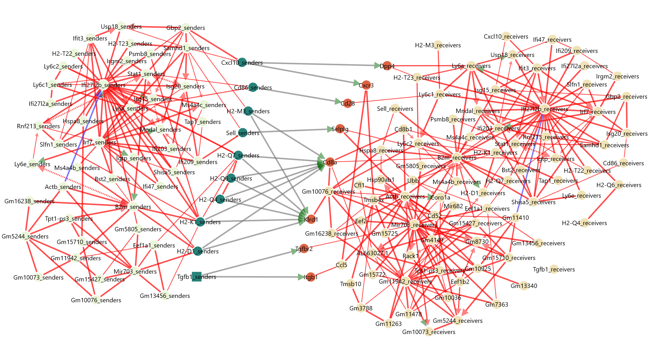
write.table(interact_edges, file.path(wd_path,"v1","MIIC_networks/causalCCC_interactEdges.tsv"), row.names=F, quote=F, sep="\t")Results